Fourier Series


Any square integrable function function, $f(x)$, in the interval $\left[-\pi,\pi\right]$ can be expressed as, \begin{equation}f(x)=\sum_{n=0}^{\infty}a_{n}\cos nx\:+\sum_{n=1}^{\infty}b_{n}\sin nx\,,\end{equation} where the constants $a_{n}$ and $b_{n}$ are given by, \begin{eqnarray} a_{n}&=&\frac{1}{\pi}\,\int_{-\pi}^{+\pi}f(x)\,\cos nx\,dx\qquad n\geq0\, \\ b_{n}&=&\frac{1}{\pi}\,\int_{-\pi}^{+\pi}f(x)\,\sin nx\,dx\qquad n>0\, \end{eqnarray} This representation of function $f(x)$ is called the Fourier series.

Problem 1

Express the function \begin{equation} f(x)=\left\{ \begin{array}{cc} +1 & \left(x<0\right)\\ -1 & \left(x\geq0\right) \end{array}\right. \end{equation} In Fourier series.

The coeffients $a_{n}$ and $b_{n}$ can be determined by the above eq.
\begin{eqnarray} a_{0}&=&\frac{1}{\pi}\int_{-\pi}^{0}(-1)\,dx\,+\,\frac{1}{\pi}\int_{0}^{+\pi}(+1)\,dx=0, \\ a_{n}&=&\frac{1}{\pi}\int_{-\pi}^{0}(-\cos nx)\,dx\,+\,\frac{1}{\pi}\int_{0}^{+\pi}(+\cos nx)\,dx=0, \\ b_{n}&=&\frac{1}{\pi}\int_{-\pi}^{0}(-\sin nx)\,dx\,+\,\frac{1}{\pi}\int_{0}^{+\pi}(+\cos nx)\,dx \\ \,&=&\frac{2}{\pi}\int_{0}^{\pi}\sin nx\,dx\quad=\;\left\{ \begin{array}{cc} \frac{4}{n\pi} & \left(n=\mathrm{odd}\right)\\ 0 & \left(n=\mathrm{even}\right) \end{array}\right. \end{eqnarray} The function $f(x)$ can be written as,$$f(x)=\frac{4}{\pi}\sum_{n=\mathrm{odd}}^{\infty}\frac{1}{n}\,\sin nx $$ or $$f(x)=\frac{4}{\pi}\sum_{n=\mathrm{0}}^{\infty}\frac{1}{2n+1}\,\sin (2n+1)x $$ The plot of series by taking different number to terms are shown in figure
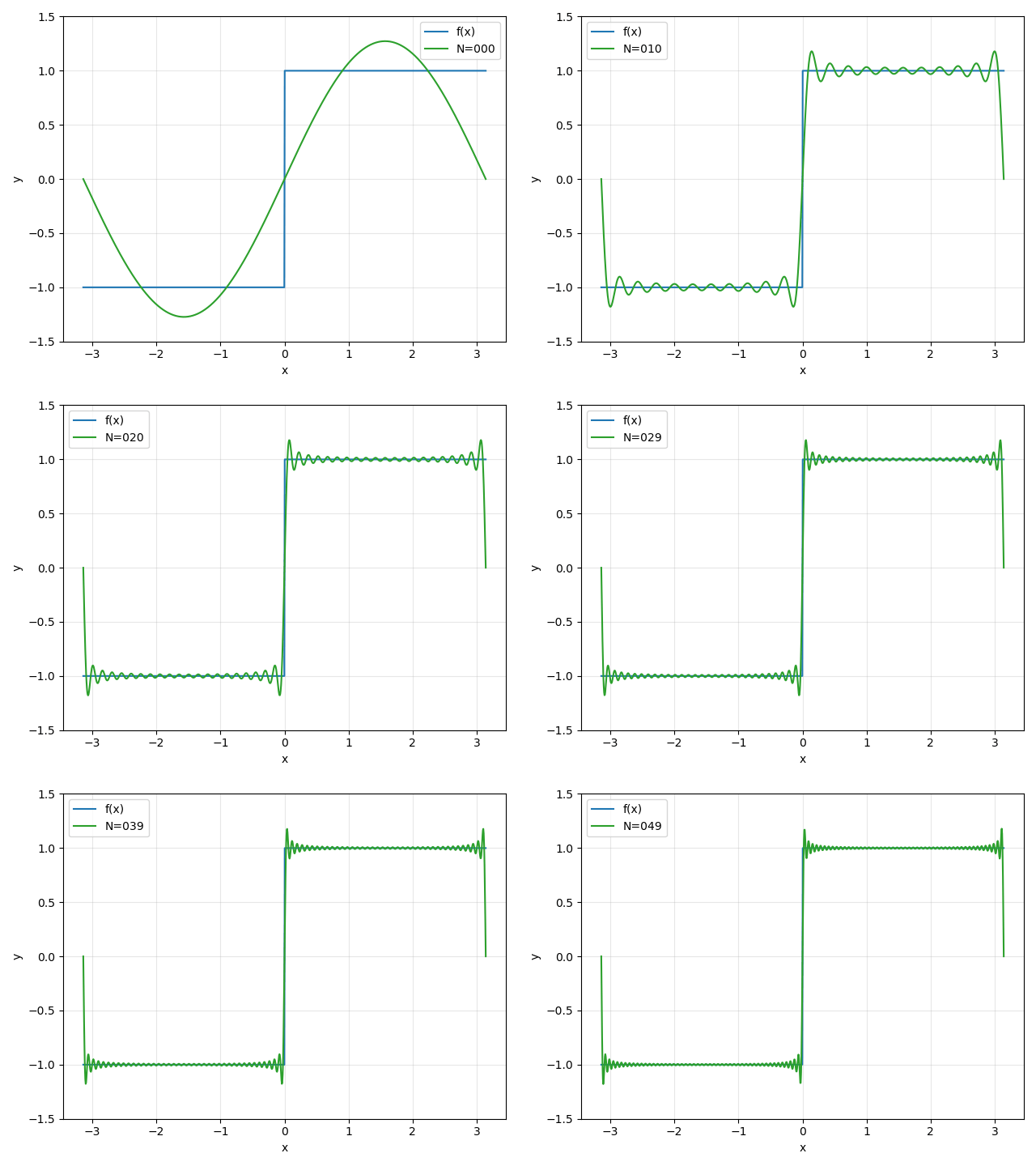
In [44]:
import numpy as np
import matplotlib.pyplot as plt
import imageio
import os
from IPython.display import Image
def f(x) :
    fx=np.ones(x.shape)
    (idx,)= np.where( x < 0 )
    fx[idx]=-1
    return fx
    
x=np.linspace(-np.pi, np.pi, 1000)
fx=f(x)


infinity=50
filenames=[]
images = []
fourierf=np.zeros(x.shape)
for n in range(infinity) :
    t1=4/np.pi * 1/(2*n+1) * np.sin((2*n+1)*x)
    fourierf+=t1
    plt.plot(x, fx, 'C0', label='f(x)')
    plt.plot(x, fourierf, 'C2',label='N='+str(n).rjust(3,'0') )
    plt.grid(alpha=0.3)
    plt.xlabel('x')
    plt.ylabel('y')
    plt.xlim([ -1.1*np.pi, 1.1*np.pi])
    plt.ylim([-1.5, 1.5])
    plt.legend()
    plt.tight_layout()
    
    fname='Fourier_'+str(n).rjust(3,'0')+'.png'
    plt.savefig(fname)
    filenames.append(fname)
    plt.close()

for filename in filenames:
            images.append(imageio.v3.imread(filename))
imageio.mimsave('Step_Fourier_Series.gif', images, duration=1)
for filename in filenames:
    os.remove(filename)
Image(url='Step_Fourier_Series.gif') 
Out[44]:

Problem 2

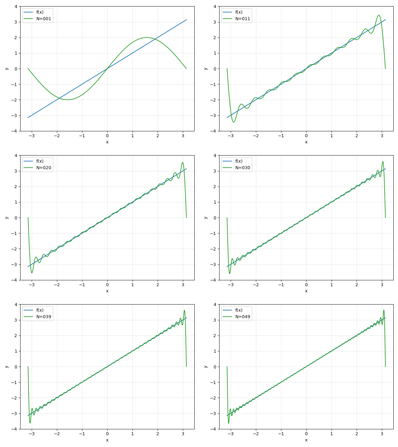
Express the function $f(x)=x\qquad-\pi<x<\pi $ in terms of Fourier series. \begin{eqnarray} a_{0}&=&\frac{1}{\pi}\int_{-\pi}^{\pi}x\,dx=0 \\ a_{n}&=&\frac{1}{\pi}\int_{-\pi}^{\pi}x\,\cos nx\:dx=0 \\ b_{n}&=&\frac{1}{\pi}\int_{-\pi}^{\pi}x\,\sin nx\:dx=-\frac{2\pi}{n}\,\cos n\pi \\ \,&=&\frac{2}{n}\,\left(-1\right)^{n+1} \end{eqnarray} and the function can be written as: $$f(x)=2\sum_{n=1}^{\infty}\left(-1\right)^{n+1}\frac{\sin nx}{n}\,.$$ The polts of various terms of this series is shown in figure

In [43]:
import numpy as np
import matplotlib.pyplot as plt
import imageio
import os
from IPython.display import Image
def linear(x) :
    fx=np.copy(x)
    return fx
    
x=np.linspace(-np.pi, np.pi, 1000)
fx=linear(x)


infinity=50
filenames=[]
images = []
fourierf=np.zeros(x.shape)
for n in range(1,infinity) :
    t1=2 * 1/n * np.sin(n*x) *(-1)**(n+1)
    fourierf+=t1
    plt.plot(x, fx, 'C0', label='f(x)')
    plt.plot(x, fourierf, 'C2',label='N='+str(n).rjust(3,'0') )
    plt.grid(alpha=0.3)
    plt.xlabel('x')
    plt.ylabel('y')
    plt.xlim([ -1.1*np.pi, 1.1*np.pi])
    plt.ylim([-4, 4])
    plt.legend()
    plt.tight_layout()
    
    fname='Fourier_'+str(n).rjust(3,'0')+'.png'
    plt.savefig(fname)
    filenames.append(fname)
    plt.close()

for filename in filenames:
            images.append(imageio.v3.imread(filename))
imageio.mimsave('Linear_Fourier_Series.gif', images, duration=1)
for filename in filenames:
    os.remove(filename)
Image(url='Linear_Fourier_Series.gif')
Out[43]:

Extended domain

The Fourier series can be extended to artitrary interval $\left[-\pi,\,\pi\right]$ to $\left[-L,\,L\right]$ by scaling. Any $L^{2}$ function in ter interval $\left[-L,\,L\right]$ can be expressed in terms of Fourier series as given in eq above \begin{equation} f(x)=\sum_{n=0}^{\infty}a_{n}\cos nx\,+\,\sum_{n=1}^{\infty}b_{n}\sin nx\,. \end{equation} where the coeffients $a_{n}$ and $b_{n}$ are given by, \begin{eqnarray} a_{n}&=&\frac{1}{L}\int_{-L}^{+L}\:f(x)\:\cos\left(\frac{n\pi x}{L}\right)\,dx\,,\\ b_{n}&=&\frac{1}{L}\int_{-L}^{+L}\:f(x)\:\sin\left(\frac{n\pi x}{L}\right)\,dx\, \end{eqnarray} An even function $f(x)$ is such that, $f(x)=f(-x)\,.$ For example $\cos x $ is an even function. An odd function is such that $f(x)=-f(x)\,.$The function $\sin x$ is an example for odd function. An even function can be expaned in Fourier cosine series and coeffients $b_{n}$ will be zero. An odd function can be expanded in terms of Fourier sine seires and the coeffients $a_{n}$ will be identically zero.

Problem

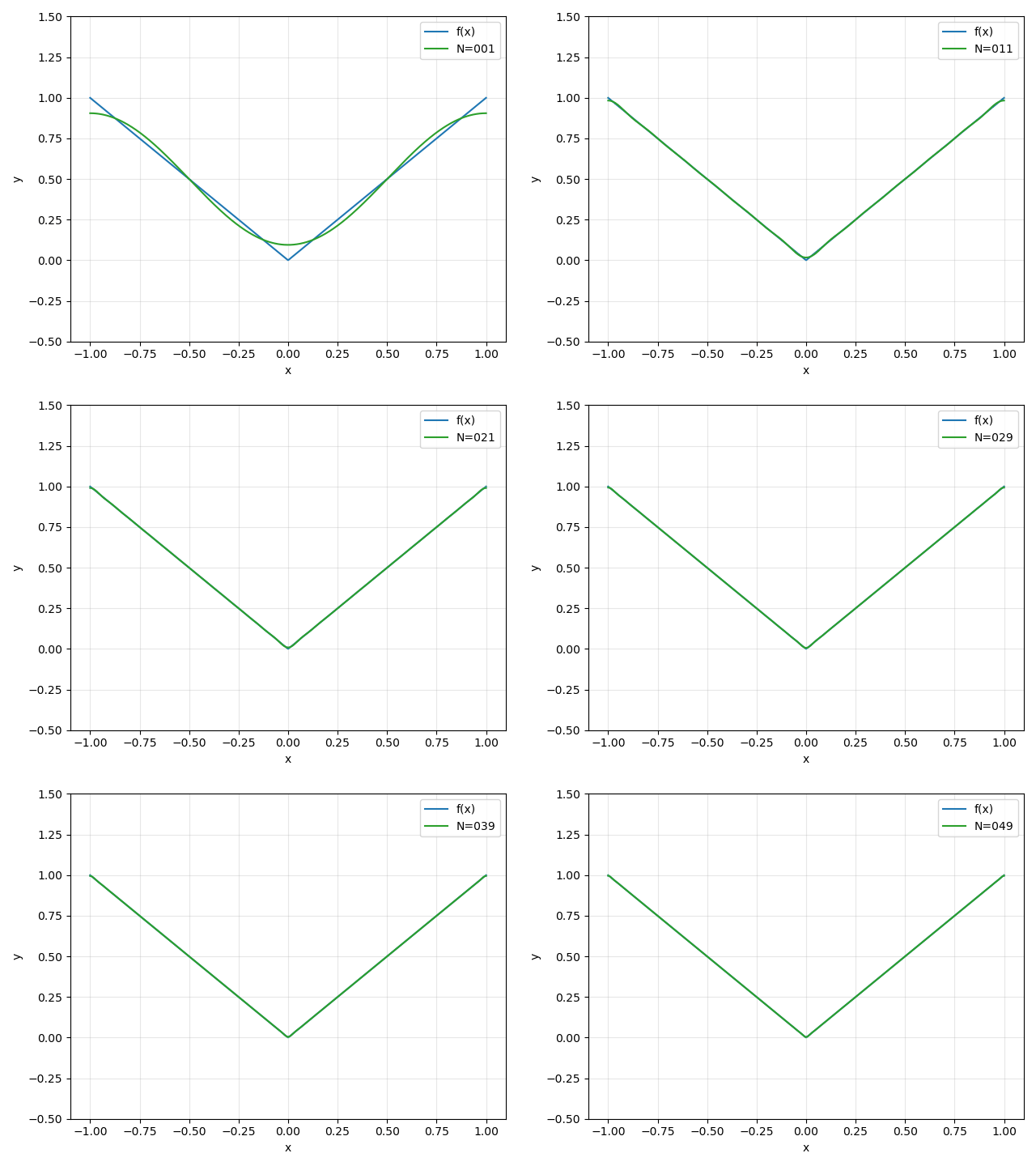
Express the function $$f(x)=\left\{ \begin{array}{cc} x & 0<x<L\\ -x & -L<x<0 \end{array}\right.$$ Since the function is an even function, the coeffients $b_{n}$ are identically zero, after simple computation, we get: \begin{equation} f(x)=\frac{L}{2}\,-\,\frac{4}{L}\,\sum_{n=\mathrm{odd}}^{\infty}\:\frac{\cos\left(\frac{n\pi x}{L}\right)}{(\pi n)^{2}}\,, \end{equation} and the plots are given in the figure

In [24]:
import numpy as np
import matplotlib.pyplot as plt
import imageio
import os
from IPython.display import Image
def absx(x) :
    fx=np.abs(x)
    return fx
L=1.0 
x=np.linspace(-L, L, 1000)
fx=absx(x)


infinity=50
filenames=[]
images = []
fourierf=np.ones(x.shape)*L/2
for n in range(1,infinity,2) :
    t1=-4/L*np.cos(n*np.pi*x/L)/n/n/np.pi/np.pi
    fourierf+=t1
    plt.plot(x, fx, 'C0', label='f(x)')
    plt.plot(x, fourierf, 'C2',label='N='+str(n).rjust(3,'0') )
    plt.grid(alpha=0.3)
    plt.xlabel('x')
    plt.ylabel('y')
    plt.xlim([ -1.1*L, 1.1*L])
    plt.ylim([-.5, 1.5])
    plt.legend()
    plt.tight_layout()
    
    fname='Fourier_'+str(n).rjust(3,'0')+'.png'
    plt.savefig(fname)
    filenames.append(fname)
    plt.close()

for filename in filenames:
            images.append(imageio.v3.imread(filename))
imageio.mimsave('Abs_Fourier_Series.gif', images, duration=1)
for filename in filenames:
    os.remove(filename)
Image(url='Abs_Fourier_Series.gif')
Out[24]:

Problem

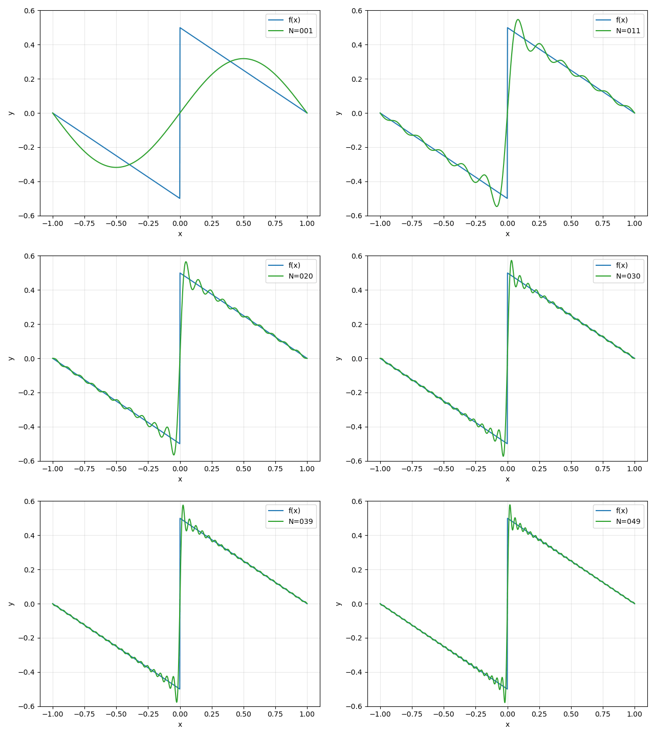
Give Fourier series expansion for the function$$f(x)=\left\{ \begin{array}{cc} \,\frac{1}{2}\left(L-x\right) & \left(0<x<L\right)\\ -\frac{1}{2}\left(L+x\right) & -L<x<0 \end{array}\right.$$ The Fourier series expansion is given by \begin{equation} f(x)=\sum_{n=1}^{\infty}\frac{1}{\pi n}\,\sin\left(\frac{n\pi x}{L}\right) \end{equation} The plots are given in the figure

In [28]:
import numpy as np
import matplotlib.pyplot as plt
import imageio
import os
from IPython.display import Image
def halflx(x, L) :
    fx=0.5*(L-x)
    (idx,)=np.where(x<0);
    fx[idx]=-0.5*(L+x[idx])
    return fx
    
    
L=1.0 
x=np.linspace(-L, L, 1000)
fx=halflx(x,L)


infinity=50
filenames=[]
images = []
fourierf=np.zeros(x.shape)
for n in range(1,infinity) :
    t1= 1/n/np.pi * np.sin(n*np.pi*x/L)
    fourierf+=t1
    plt.plot(x, fx, 'C0', label='f(x)')
    plt.plot(x, fourierf, 'C2',label='N='+str(n).rjust(3,'0') )
    plt.grid(alpha=0.3)
    plt.xlabel('x')
    plt.ylabel('y')
    plt.xlim([ -1.1*L, 1.1*L])
    plt.ylim([-.6, .6])
    plt.legend()
    plt.tight_layout()
    
    fname='Fourier_'+str(n).rjust(3,'0')+'.png'
    plt.savefig(fname)
    filenames.append(fname)
    plt.close()

for filename in filenames:
            images.append(imageio.v3.imread(filename))
imageio.mimsave('Halflx_Fourier_Series.gif', images, duration=1)
for filename in filenames:
    os.remove(filename)
Image(url='Halflx_Fourier_Series.gif')
Out[28]:

Dirac $\delta$

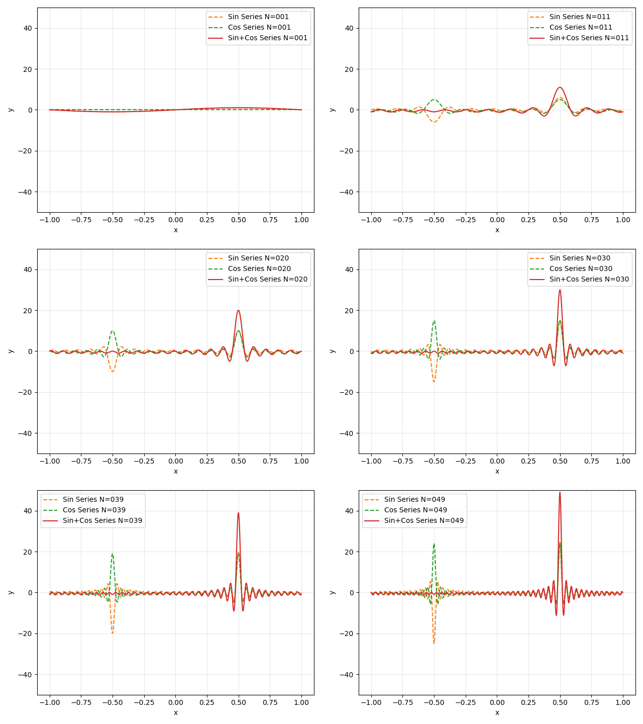
The Dirac delta function $\delta\left(x-x'\right)$ is such that, \begin{equation} f(x')=\int_{a}^{b}f(x)\,\delta(x-x')\,dx=\left\{ \begin{array}{cc} f(x') & x'\in\left[a,b\right]\\ 0 & x'\notin\left[a,b\right] \end{array}\right. \end{equation} can be expressed in terms of Fourier seires as follows \begin{eqnarray} \delta\left(x-x'\right)&=& S+ C \\ S& = &\left(\frac{1}{L}\right)\sum_{n=1}^{\infty}\sin\left(\frac{n\pi x}{L}\right)\sin\left(\frac{n\pi x'}{L}\right)\,, \nonumber \\ C & = & \left(\frac{1}{L}\right)\sum_{n=0}^{\infty}\cos\left(\frac{n\pi x}{L}\right)\cos\left(\frac{n\pi x'}{L}\right)\,, \end{eqnarray} where $L=b-a$. The coeffients $\left\{ a_{n},\,b_{n}\right\}$ can easily determined

In [32]:
import numpy as np
import matplotlib.pyplot as plt
import imageio
import os
from IPython.display import Image
L=1.0 
x=np.linspace(-L, L, 1000)
xp=0.5
infinity=50
filenames=[]
images = []
deltaS=np.zeros(x.shape)
deltaC=np.zeros(x.shape)
for n in range(1,infinity) :
    s1= 1/L * np.sin(n*np.pi*x/L)*np.sin(n*np.pi*xp/L)
    c1= 1/L * np.cos(n*np.pi*x/L)*np.cos(n*np.pi*xp/L)
    deltaS+=s1
    deltaC+=c1
    
    plt.plot(x, deltaS, 'C1--',label='Sin Series N='+str(n).rjust(3,'0') )
    plt.plot(x, deltaC, 'C2--',label='Cos Series N='+str(n).rjust(3,'0') )
    plt.plot(x, deltaS+deltaC, 'C3',label='Sin+Cos Series N='+str(n).rjust(3,'0') )
    plt.grid(alpha=0.3)
    plt.xlabel('x')
    plt.ylabel('y')
    plt.xlim([ -1.1*L, 1.1*L])
    plt.ylim([-50,50])
    plt.legend()
    plt.tight_layout()
    
    fname='Fourier_'+str(n).rjust(3,'0')+'.png'
    plt.savefig(fname)
    filenames.append(fname)
    plt.close()

for filename in filenames:
            images.append(imageio.v3.imread(filename))
imageio.mimsave('Delta_Fourier_Series.gif', images, duration=1)
for filename in filenames:
    os.remove(filename)
Image(url='Delta_Fourier_Series.gif')
Out[32]:
In [ ]: