Heavy rains have hit the city; once in a quiet afternoon they may drizzle or storm down to the ground in an ode to joy. The sweltering heat would stand back in awe of their little mysteries, their insightful selves and gargantuan potential. Their faint rhythm would overflow the serene countryside and dissolve the neon cityscape. Pura slowly climbed the stairs as Senn guided her. She was working quite a bit and was supposed to rest, but this day was so important to her. She would be excited to hold the session each month, despite not having much vis-a-vis interaction.
“Good evening, all my friends and family! We meet again to look at some wonderful ideas and try to put our finger on a few nice problems. It is very unfortunate that I am not doing my best right now, although I am not in any trouble. Nevertheless, if I do feel like resting my voice for a bit, Senn will be glad to take over. I’m sure you’ll show him the same love you have shown me.
Our thing of interest today are errors. Indeed as they say - To err is human, for no err is of whom but supreme? However, accepting our errors makes our convictions stronger and our ideas more robust; that is how science has progressed all this while. Let us get to today’s problems.
We often hear scientists approximating a curve to a straight line - does that even work? Well, we know from calculations that the Earth is round - I mean, somewhat; however when you look down the street it is a straight road. In fact, some roads are so straight you wouldn’t even find small bumps in them. This means that a very small portion of a curved/spherical surface is akin to a plane. Similarly, a small portion of a curve is akin to a straight line. There is indeed some error in accuracy, generally too small to see. Our aim is to look at this error and determine how fast it grows as our portion of the curve grows in size.
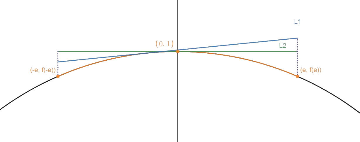
Figure 1. A small arc of the upper half of the unit circle approximated by two straight lines $L_1$ and $L_2$. The extreme coordinates are as $(\pm \epsilon, f(\pm \epsilon))$, where $\epsilon$ is a small number as compared to the radius - in the figure it is exaggerated.
In Figure 1, there are two straight lines that approximate a small epsilon arc ($-\epsilon\leq x\leq \epsilon$) of the upper half of the unit circle $x^2+y^2=1$. $L_2$ is tangent to the circle at its maxima i.e. at $x=0$, while $L_1$ is tangent at some other point. We may often think which one of $L_1$ or $L_2$ is a better linear approximation for the arc (note that the image is exaggerated for clarity and in reality $\epsilon\ll 1$). The way in which we shall understand accuracy here is by a length error, which is
\[\Delta_{ac}=|l_c-l_{ac}|\]where $l_c$ is the length of the curve in the given interval and $l_{ac}$ is the length of the approximated curve (a straight line in this case) in the given interval. Let me put one part down: the highlighted length of $L_2$ is basically the difference of the abscissa of the extrema, and hence
\[l_{L_2}=\epsilon-(-\epsilon)=2\epsilon.\]What about the arc length? We know that if the radius $r$ (which is 1 here) subtends an angle $\theta$ on an arc, then the length of the arc is given by $r\theta$ ($=\theta$ in this case). Can you somehow relate $\theta$ with $\epsilon$? Also, can you compare the length of $L_1$ to $L_2$?
(i) Give a geometric explanation as to why $l_{L_2}\leq l_{L_1}$.
(ii) Give an algebraic argument for the same.
Could you work them out? Now, many of you might be thinking that $L_1$ might be a better approximator of the arc than $L_2$, if the length error $\Delta_{L_1}<\Delta_{L_2}$. However, since the curve is centred around zero, and $\epsilon$ is really small, we are actually looking at an approximation of the curve/arc in an $\epsilon$-neighbourhood of zero, where $\epsilon\to 0$. Then, our linear approximation is called an affine approximation at $x=0$. The best affine approximation is extracted from a set of rules; we are only interested in the tangency of the straight line at the point of approximation. Clearly, $L_2$ is the best candidate which is tangent to the curve at our central point $x=0$, so it is the best affine approximator of our arc. Not satisfied? Well, at least it is a better economic choice; $L_2$ having the smallest length would cost the least money/labour if you were assigned to construct it!
Now that we are done with the fundamental idea, let’s move on to some math!” Pura stopped to take a breath. “Is it fine if I go forward with it, Pura?” Senn asked from the couch.
“Sure, let me just visit the restroom and you can continue for a while.” she replied and smiled reassuringly. “I’m the best I can.”
“Cool.” Senn smiled back. “Okay, so we come to the math part - which is once again something that I like toying around with. We will be looking at smooth functions today, also known as belonging to $C^{\infty}$. These functions are infinitely differentiable, and all derivatives are by definition continuous. Another property we would use is that these functions are analytic, or in $C^{\omega}$, which means that a Taylor series expansion of this function in the neighbourhood of a point will always converge to the functional value at that point.
So, what is a Taylor series?
Well, if you have a smooth function analytic about some point $x=a$, then we can expand $f(x)$ around that point as
\[f(x)=f(a)+f'(a)(x-a)+f''(a)\frac{(x-a)^2}{2!}+f'''(a)\frac{(x-a)^3}{3!}+\ldots\]which is a really simple construction. We are also happy with a Taylor series as long as the infinite sum converges to a finite value - and we shall assume all our functions do that unless explicitly mentioned.
Did you know that if $a=0$ in a Taylor series expansion, it is better known as a Maclaurin series? Since most of our problems will be centred around $x=0$, we can just call them Maclaurin series. Let me provide an example to help you better; let us take $f(x)=\sin(x)$, then
\[\begin{align*} f'(x)&=\cos(x)\\ f''(x)&=-\sin(x)\\ f'''(x)&=-\cos(x)\\ f''''(x)&=\sin(x)\\ .\\ .\\ . \end{align*}\]Thus the derivatives form a periodic sequence of sinusoidal functions. Now if you were to write the Maclaurin series of $\sin(x)$ by setting $a=0$ in the above definition of the Taylor series, you would get
\[\sin(x)=x-\frac{x^3}{3!}+\frac{x^5}{5!}-\frac{x^7}{7!}+\ldots\]Maclaurin series of some other common functions are
\[\cos(x)=1-\frac{x^2}{2!}+\frac{x^4}{4!}-\frac{x^6}{6!}+\ldots\] \[e^x = 1+x+\frac{x^2}{2!}+\frac{x^3}{3!}+\ldots\] \[\ln(1+x)=x-\frac{x^2}{2}+\frac{x^3}{3}-\frac{x^4}{4}+\ldots\hspace{0.15 in}\text{for }|x|<1\]We would extensively use these series when trying to compute the length errors for our approximations.
Now let us go back to our original problem. Designate $L_2\to L$ and then we have
\[\Delta_L = l_c-l_L=l_c-2\epsilon\]Use the series
\[\sin^{-1}(x)=x+\frac{x^3}{6}+\frac{3x^5}{40}+o(x^7)\]for $|x|<1$ to compute $\Delta_L$ and find out the smallest power of $x$ in it. Note that $o(x^n)$ in layman terms means that there are higher powers of the order $x^n$ or even higher, e.g. $x+x^3+x^5+x^7+\ldots=x+o(x^3)=x+x^3+o(x^5)$ and so on. For example, if $\Delta_L=Ax^2+Bx^5+Cx^7+o(x^8)$, then the smallest power is that of $x^2$. This smallest power is also defined as the growth factor of the error.
(iii) What is the growth factor of $\Delta_L$ in this case?
Some of you might be thinking - why is the smallest power designated as the growth factor if we have higher powers? Do note that we set $\epsilon\ll 1$, so the higher the power $k$ we take, the smaller $\epsilon^k$ becomes. So the growth factor of the length error as $\epsilon$ increases is dominated by the smallest index term.”
Pura was already back and had seated herself comfortably. “I’ll take from here”, she said softly, positioning herself properly.
“So now that you probably have calculated the error growth for a linear approximation of a circular arc, let’s try some other curves; for a given I’ll take them to be nice and symmetric.
Consider a general curve $f(x)$ which is smooth and analytic, and we have $f(0)=1$ and an affine approximation at $x=0$ extended to the interval $(-\epsilon,\epsilon)$. Then the length of the line is given by $l_L=2\epsilon$. The length of the curve however, is not so trivial to compute. In fact, it somewhat relies on the fact that infinitesimal curve segments are indistinguishable from a line if the curve is smooth and has a nonzero derivative. Suppose we have an element $ds$ of a curve as shown in Figure 2.
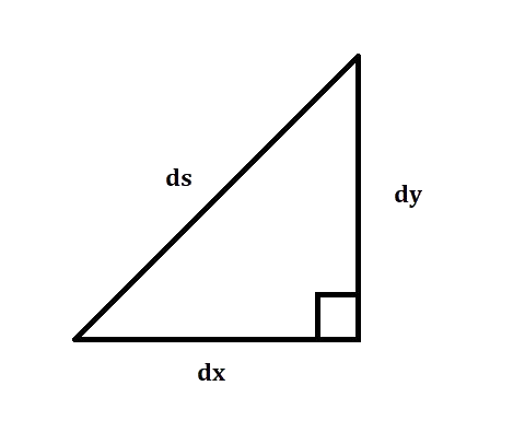
Figure 2. We look at an infinitesimal element $ds$ on a curve. From Pythagoras’ theorem we have $dx^2+dy^2=ds^2$. In fact, this is a property of the Euclidean metric where the distance between a pair of points is just their straight line separation and Pythagoras’ theorem applies here.
Clearly for an entire curve in $I=(-\epsilon, \epsilon)$, the length of the curve is the sum of all such $ds$ elements; which can be written down in a clever fashion as
\[l_c=\int_Ids=\int_I \sqrt{dx^2+dy^2}=\int_I\sqrt{1+\left(\frac{dy}{dx}\right)^2}dx=\int_{-\epsilon}^{\epsilon}\sqrt{1+y'^2}dx\]As long as the integral converges, we can find $l_c$ and hence $\Delta_L$. Let us try a problem with the parabola $y=1-x^2$.
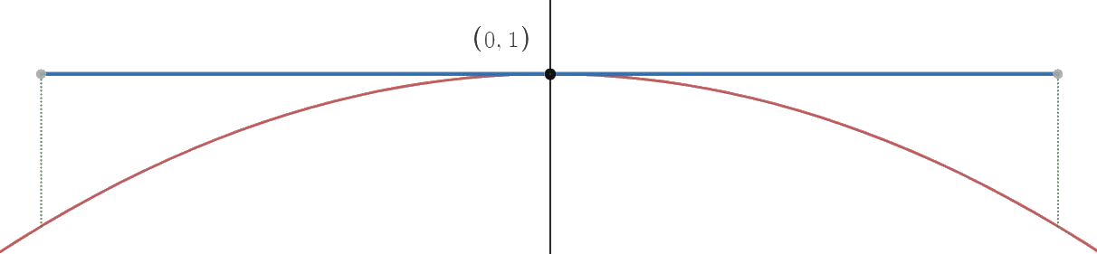
Figure 3. A linear approximation for the given parabola $y=1-x^2$ in the $\epsilon$ neighbourhood of $x=0$.
It is easy to compute that $y’=2x$ and so
\[\Delta_c = \int_{-\epsilon}^{\epsilon}\sqrt{1+4x^2}\text{ }dx-2\epsilon\]We wish to look at the growth factor of $\Delta_L$ now. Note that it won’t be easy to Taylor expand every term so try using the $o()$ notation and only work with the first few terms. You can use the binomial expansion for $|x|<1$
\[\sqrt{1+x}=1+\frac{x}{2}-\frac{x^2}{4}+\frac{3x^2}{8}+o(x^4)\](iv) Find the growth factor (smallest power of $\epsilon$) of $\Delta_L$.
(v) Is the growth in this case slower than that for the circle? Explain.
We can try another curve - the hyperbolic cosine function, given as
\[\cosh(x)=\frac{e^x+e^{-x}}{2}\]Our function would go as $f(x)=2-\cosh(x)$ (often called a catenary) so that it takes the maximum value of $1$ at $x=0$. Once again, the approximated line is of length $2\epsilon$ and is tangent to the curve at $x=0$, and we want the growth factor of $\Delta_L$.
(vi) What is the growth factor of $\Delta_L$ in this case (show it) and how does it compare to those for a parabola and a circle.
These are three very nice examples where we get an estimate of errors in approximation.”
“The reason why we can’t just give you a list of curves” Senn walked up to the front, “is because most curves do not have a closed form for the arc length. They give what is known as an elliptic integral. A cool example is the arc length about $f(x)=\cos(x)$ around $x=0$; the path length integral to solve would be
\[l_c = \int_{-\epsilon}^{\epsilon}\sqrt{1+\sin^2(x)}dx\]Can you solve this integral in a closed form? Give it a try when you’re feeling bored and intelligent!
Moving on, we can take a look at errors in computation as well. Often a problem posed at hand is too complicated or difficult to be solved by hand; we need computers for that. Since computers can’t work with abstract quantities like infinitesimals or infinite sets, we generally use discrete approximation of the underlying math. One of the uses is to numerically calculate the derivative of a differentiable function.
Consider a smooth analytic function $f(x)$ that has a convergent Taylor expansion everywhere. We will check three different finite difference methods to calculate the derivative and find out the best method from the relative growth factors of the error. Here, we define our error to be a distance error
\[\Delta_{\delta}=\left|f'(x)-\delta f(x)\right|\]where $\delta/\delta x$ is our numerical derivative calculator.
The three methods that we shall now state are as follows ($h\ll 1$):
- Standard Method : $\delta_1f(x)=\frac{f(x+h)-f(x)}{h}$
- Symmetric Difference Method : $\delta_2f(x)=\frac{f(x+h)-f(x-h)}{2h}$
- Five point method : $\delta_3f(x)=\frac{-f(x+2h)+8f(x+h)-8f(x-h)+f(x-2h)}{12h}$
As mentioned earlier, the Taylor series can be written as
\[\begin{align*} f(x+h)=f(x)+xf'(x)+\frac{x^2}{2!}f''(x)+\frac{x^3}{3!}f'''(x)+\ldots\\ f(x-h)=f(x)-xf'(x)+\frac{x^2}{2!}f''(x)-\frac{x^3}{3!}f'''(x)+\ldots \end{align*}\](vii) Find the growth factors for the three methods and find the best approximation.
(viii) Mention any drawbacks that the best approximation has as compared to the other two.
Aren’t the results you derived interesting? Why do you think that something as elementary as computing a derivative would see a major difference in error accuracy just by cleverly changing the method? Indeed, the entirety of science and computation is filled with such examples. There are many places where the rudimentary way of performing a computation is often less accurate and time consuming. Scientists then come up with alternate ways that provide a better approximation in a shorter computation time. As I like to say, The world of first principles is mathematical, the rest are simply logical.”
“Wasn’t this a long session?” Pura retorted gleefully. “Even I had to take a break since so much stuff was going on. I would love to continue on this today, especially with statistical and sampling errors - however time is running out and introducing another new concept would be somewhat hefty; so I’ll just gloss over a couple easy ones before ending for today.
Errors on perturbation of the argument of a function is very prevalent in physics - one that we have to use a lot in experiments. The main idea of it is that a positive error in the tuner $x$ translates to the output $f(x)$ which we consider to be smooth and analytic. Note that the translation might not be positively correlated with the error. In general
\[f(x+\Delta x)=f(x)+\Delta_{\Delta x}\]where $\Delta x>0$. Take $\Delta x=\epsilon\ll 1$. Now let us look at some problems. Note $x>0$.
- $\sin(x+\epsilon)=\sin(x)+\Delta_{\epsilon}$
- $\ln(x+\epsilon)=\ln(x)+\Delta_{\epsilon}$
- $\frac{1}{x+\epsilon}=\frac{1}{x}+\Delta_{\epsilon}$
- $f(x+\epsilon_x,y+\epsilon_y,z+\epsilon_z)=f(x,y,z)+\Delta_{\epsilon_1,\epsilon_2,\epsilon_3}$ where $f(x,y,z)=\frac{xy}{z^2}$
You may use the negative binomial expansion
\[(1+x)^{-n}=1-nx+\frac{(-n)(-n-1)x^2}{2!}+\frac{(-n)(-n-1)(-n-2)x^3}{3!}+\ldots\]as well as the multivariable Taylor expansion
\[\begin{align*} &f(x+h_x,y+h_y,z+h_z)\\ &= f(x,y,z)+h_x\frac{\partial f}{\partial x}+h_y\frac{\partial f}{\partial y}+h_z\frac{\partial f}{\partial z}+\frac{h_x^2}{2!}\frac{\partial^2 f}{\partial x^2}+\frac{h_y^2}{2!}\frac{\partial^2 f}{\partial y^2}+\frac{h_z^2}{2!}\frac{\partial^2f}{\partial z^2}+\ldots \end{align*}\]where $\partial/\partial z$ is the partial derivative w.r.t z, i.e. all other variables are treated as constants. E.g.
\[\frac{\partial}{\partial z}(x+yz)=0+y\frac{\partial}{\partial z}z=y\]Now that you’ve got the requirements, dive in!
(viii) Find out the growth factors in each of the $\Delta_{\epsilon}$ for the three univariate functions given above and compare them.
(ix) Find the growth factors of $\epsilon_1$, $\epsilon_2$, $\epsilon_3$ in the trivariate function given and compare them.
For the trivariate function, can you see how we do first order approximations (a.k.a only retaining terms of order $\sim \epsilon^1$) to calculate percentage error in the quantity during error analysis in experiments?”
“So, we are a minute overtime Pura.” Senn got up, looking at his watch. “You shouldn’t be over-working, right?”
Pura chuckled to herself. “Are you worried eh? Okay, let’s go.”
“Well, I should be, right? Besides, this was a really long session since you probably included some of next month’s work in here too. Now I have to design some other idea I guess…”
“Nah, I’ll do it myself. Don’t you have like, work? You probably will be away for a while, duh.”
“Yea we’ll talk about it tomorrow - let’s draw the curtains today with four lines I wrote, how ‘bout that?”
“Go on, go on! Are they as goofy as you said they’d be; I’m curious!”
To err is to human, to forgive divine
The err seen in Newton, fixed by Einstein
Err of the axioms make poor Euclid cry
Err in the car brakes may help one man die.
Submitting
Send in your solutions at maths.club@iiserkol.ac.in.